An Introduction to Reinforcement Learning

Recent successes, achieved with the help of Reinforcement Learning, have quite extensively been covered by the media. One can think of DeepMind’s AlphaGo algorithm: Using Reinforcement Learning (and a massive amount of expensive hardware to train it), AlphaGo learned to play the age-old game of Go and even developed its own playstyle.

Another example was demonstrated by OpenAI, whose researchers taught a robot hand to solve a Rubik’s Cube. The interesting aspect is that it was trained in a virtual environment; and because even holding and turning around a cube without dropping it is quite hard, this is an amazing first step.

My intention with this post is to explain the concepts that make such successes possible in the first place. I start with an introduction, and then progressively refine the definition of RL.

Introduction

Reinforcement learning (RL) is an area of machine learning. You might have already worked with supervised learning (where the data is labelled), and unsupervised learning (unlabeled data, e.g., for generative techniques). These two broad fields are complemented by the domain of reinforcement learning. Two key differences are that the data is usually not independently and identically distributed (i.e., it can be quite messy with no apparent structure), and that an agent’s behaviour determines the future data it encounters.

In one informal sentence, Reinforcement learning learns to achieve a goal through interaction.

Let’s cover the basic ingredients behind this branch of machine learning:

At first, we have the mentioned agent. The agent is both the one that learns and the decision-maker. The real-life analogy would be you and me, who are making decisions and learning on the go. Secondly, everything that the agent can interact with is the environment (which for us would be our normal surroundings: other people, buildings, cars, dogs, cats, …). Thirdly, this environment can change through interaction, which is the agent’s only way to have an impact. In every possible situation, an agent can decide on an action and gets rewarded in turn. This reward then influences the learning process.

MDP

This description is rather vague. To come up with a more precise definition of Reinforcement Learning we need a mathematical approach. This is where the Markov Decision Process comes in, a mathematical way to model the transition between states. We have a quintuple of (S, A, R, P, p₀) [1,2]:

S is the state space and contains all possible states that an agent can encounter. Thus, every single state s ∈ S.

A is the action space, which contains the agent’s possible actions. Likewise, we have every single action a ∈ A.

R is the reward function, which delivers the reward of an agent’s action, based on the current state sₜ, the chosen action aₜ, and the resulting state sₜ₊₁. We include the resulting state to also respect the transition between states. Without it, acting in the same state at different time steps would yield the same reward — not taking into account what an agent might have learned already. In other words, the action a can be the same at t and t+k but might lead to a different new state. We take this into account by adding sₜ₊₁. A reward is a real number, such as +1, -2.5, and so on.

P is a function that maps a state and an action to a probability. It determines the probability of reaching state sₜ₊₁ when coming from sₜ and choosing action aₜ. Our environment might be influenced by events out of our control. For this reason, we have P, which takes into account external influences. If we do not have such influences, we simply use a deterministic transition, that is the new state is guaranteed to be reached.

And lastly, we have p₀, which is the distribution of the starting states, that is it contains all states that we can start from.

Do you remember the mobile game DoodleJump? Or the Mario games on the Nintendo devices? Let’s construct a setting similar to those two:

Our enemies come in from the right side (this is from Mario), and we can evade them by jumping one level up (this is from Doodle Jump). Our state space S consists of two states, low and high.

In both states we have two possible actions, jump and wait, which make up the actions space A.

Every time we jump from low to high or from high to high we get a reward of +1. When we get hit by an enemy we fall down one level, and the reward is -1 (note that here the reward is not tied to an action, such as jump or wait, but to the fact that we get hit by an external influence). Waiting has a reward of 0.

Now to P, which determines how likely we are to reach the next level. This is 80 %, with 20 % we remain on the current level. Waiting can lead with equal probability to remaining at the current level or getting hit by an enemy; the probability is thus 50 % for both. Lastly, our p₀ only contains the state low.

Policy

So far we have covered actions and environments, but not how to determine the appropriate action in a given state. Since we have multiple states and multiple time steps we need some further algorithm to help us. This is the task of the policy π, the mapping from a state to an action: π(aₜ|sₜ) is the probability of selecting aₜ in state sₜ [1,2] (you can think of a set of rules: If this then that). Going from this, we can sample actions from all possible actions, denoted by aₜ ∼ π(.|sₜ).

The policy is the part that can be modelled by neural networks in Deep RL [1].

For our example, our policy consists of the following mappings: (jump|low) = (jump|high) = 50 %. This means in the states low and high we chose the action jump with a probability of 50 %. The probabilities of (wait|low) and (wait|high) are 50 % each.

Rewards

Until now we have covered the policy, but not how the rewards look and what they do. At the start, I noted that we want the agent to achieve a goal. This is rather vague. More formally, we want the agent to maximize the expected reward.

Let’s look at this:

Going from our initial state s₀ with a₀ leads us to s₁. With a₁ we get to s₂. And with a₂ we then advance to s₃. This goes on, possibly for an infinite amount of time steps t. Such a sequence of states and actions is called a trajectory, denoted τ. Further, we also get rewarded after each action, with a reward rₜ₊₁ (since the reward takes into account the resulting state, the reward is also paid out at the next time step, t+1). With both the trajectory and the reward we can calculate our final return, or the cumulative reward, by summing over all individual rewards [1,2]

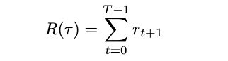
Returning to our example, consider this trajectory: (low, jump, high, jump, high). The reward for the transition from low to high is +1, and the reward from high to high is also +1. For this trajectory, the return would be 2.

In the case of a finite sequence of actions, this is all we need. But when we deal with endlessly running environments, this poses a problem:

Every reward currently has the same importance, whether it takes place at a near time step (and thus might be more tangible) or at the edge of infinity (highly intangible). Further, and this is more important, our return is not bounded, it does not converge to a fixed value. This makes it difficult to compare two policies: One might always get a return of +1, -1, +1, -1, …, whereas the other policy might frequently get +10, +10, +10, only to make a serious mistake later on that cancels all we have achieved so far. In other words, when the trajectory is endless, we don’t know which policy will be better in the long run, since everything might happen.

Luckily, this can be solved by using discounted returns, a more general approach: We multiply each reward with a discount, which quantifies its importance (setting the discount to 1 lead to the previous undiscounted return) [1,2]:

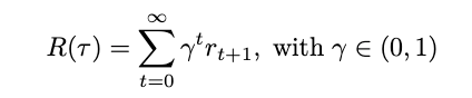
Having a discounted return thus enforces an agent to “win sooner rather than later” [3].

To maximize the expected reward we need our policy (check), our trajectory (check), and the return (check). Equipped with them we begin with:

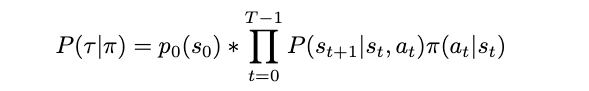
Let me explain this equation: Given a policy π, we want to know how likely it is that we get a specific sequence of states and actions (this is the trajectory, τ). For this, we take the probability of our start state s₀ and then multiply this with all further probabilities (this is the ∏ part). For each later state sₜ₊₁ that we reach we check how likely it is to reach this state (that’s the P(sₜ₊₁|sₜ,aₜ)), and multiply this with the chances of taking the action that lead us there (that’s the π(aₜ|sₜ)).

Following this, we write that the expected return is the reward that we get with a policy π and then acting accordingly to it (which gets us the trajectory, the list of state-action sequences). For each such trajectory, we have, as seen above, a return. Going over all possible trajectories (all possible state-action sequences), and summing up their individual returns, we then have our expected reward [1,2]:

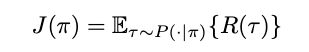
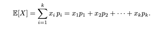
Let me cover the equation in more detail: We take each possible trajectory by writing the τ ∼ P(⋅|π). As I have written above, each trajectory has a probability of occurring, and each trajectory has a reward. By multiplying the probability with the reward (that’s described by R(τ)) we weight the result according to its likeliness. This follows the normal way to calculate the expected value:

For our example, we have these two trajectories: (low, jump, high, jump, high) (with a reward of 2), and the trajectory (low, jump, high, wait, low) (with the reward 0: +1 for advancing, -1 for waiting and getting hit by an enemy, thus falling one level).

Let’s now calculate the probability for the first trajectory: It’s 1 × 0.8 × 0.5 × 0.8 × 0.5 = 0.16; the 1 is the probability of the start state low, the 0.8 × 0.5 are the probabilities of advancing to the next level, multiplied by the probability of selecting the action jump. Similarly we proceed for the second trajectory: 1 × 0.8 × 0.5 × 0.5 × 0.5 = 0.1, the only difference is 0.5 × 0.5. Here, we take the probability of 0.5 for waiting (that is, falling one level in this case) and multiply this by the success ratio, 0.5.

With each trajectory’s reward and probability at hand, we can now calculate the expected reward by following the above equation: 0.16 × 2 + 0.1 × 0=0.32. Our expected reward is thus 0.32.

With this said, we can further formalize our RL definition: Find the policy which maximizes the expected reward [1,2]

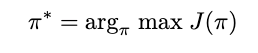
This is the optimal policy.

Value functions

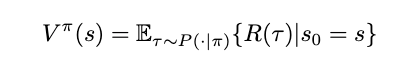
With all this said, how do we know if an action is a good action, or a state is a good state? We can find this out with value and action-value functions. Put simply, given a policy π, the value of a state is the expected return that follows from this state and always acting according to π thereafter. Using mathematical notation, we write this as

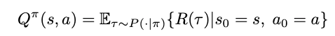
Similarly, for action-value functions, we need also the policy π. Different to before, we now assign the value to a pair of state and action [1,2]. The value is, again, the expected reward that follows when we start ins s₀ and act with a₀:

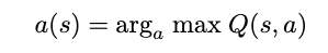
Having Q, we can then simply choose the next action for a state as the action that maximizes the expected reward

Similarly, we can check the value of a state by consulting V.

The cool thing is that with an optimal policy we can find both the optimal value and optimal action-value function. And this optimal policy always exists for any MDP. The challenge is in finding it.

References

[1] Josh Achiam, Spinning Up in Deep RL (2020), OpenAI

[2] Sutton, Richard S and Barto, Andrew G, Reinforcement learning: An introduction (2018), MIT press

[3] Michael L. Littman, Markov games as a framework for multi-agent reinforcement learning (1994), Machine learning proceedings